Tapani Pihlajamäki, Olli Santala, and Ville Pulkki
Synthesis of Spatially Extended Virtual Sources with Time-Frequency Decomposition of Mono Signals
Companion page for a paper published in the Journal of the Audio Engineering Society, Volume 62, Number 7/8
Abstract
Synthesis of volumetric virtual sources is a useful technique for auditory displays and virtual worlds. This task can be simplified into synthesis of perceived spatial extent. Previous research in virtual-world Directional Audio Coding has shown that spatial extent can be synthesized with monophonic sources by applying a time-frequency-space decomposition, i.e., randomly distributing time-frequency bins of the source signal. However, although this technique often achieved perception of spatial extent, it was not guaranteed and the timbre could degrade. In this article, this technique is revisited in detail and the effect of different parameters is examined to ultimately achieve optimal quality and perception in all situations. The results of a series of informal and formal experiments are presented here and they suggest that the revised method is very viable in many cases. There is some dependency on the signal content that warrants proper tuning of parameters. Furthermore, it is shown that different distribution widths can be produced with the method as well. From a psychoacoustical perspective, it is interesting that distributed narrow frequency bands form a spatially extended auditory event with no apparent directional focus.
Complete results
Here, the complete results are provided for the reader to analyze. This contains the separate histogram plots for different sample types in experiment 1a, all the significant effects in variance analysis of experiment 1b, and the histogram plot for experiment 2.
Results of experiment 1a
These plots show the distribution histograms for the different program material data. Blue signifies any sound and red signifies major sound. Thick gray line is the 100% marker and dotted lines are 75%, 50%, and 25% markers. The histogram is on a square-root scale as this makes areas visually comparable. Small black boxes indicate the loudspeaker directions. The bars on the right side of each histogram signify the percentage of subjects answering that the sound comes inside or near the head (left bar, violet), and from above or below (right bar, gray).
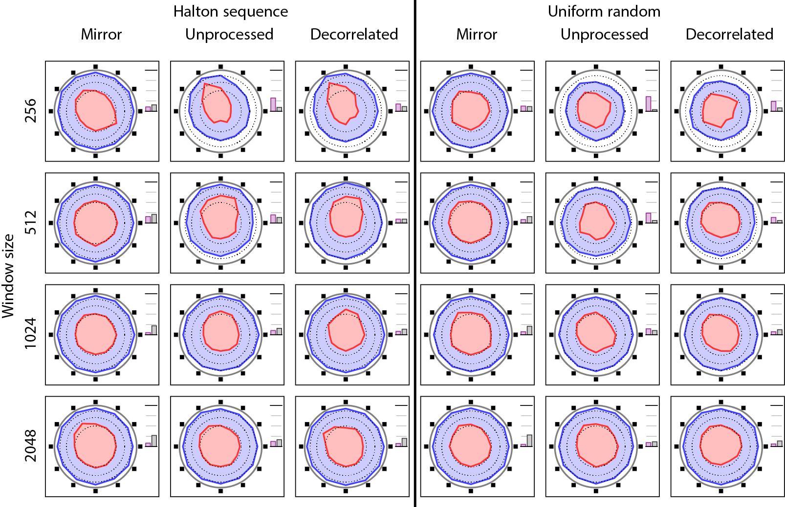
Figure: This is the combined plot presented in the paper. |
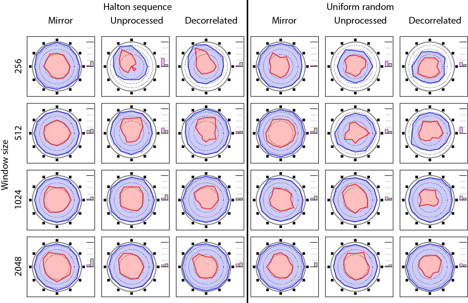
Figure: This is the result for the sample containing a cello playing in dry acoustics. |
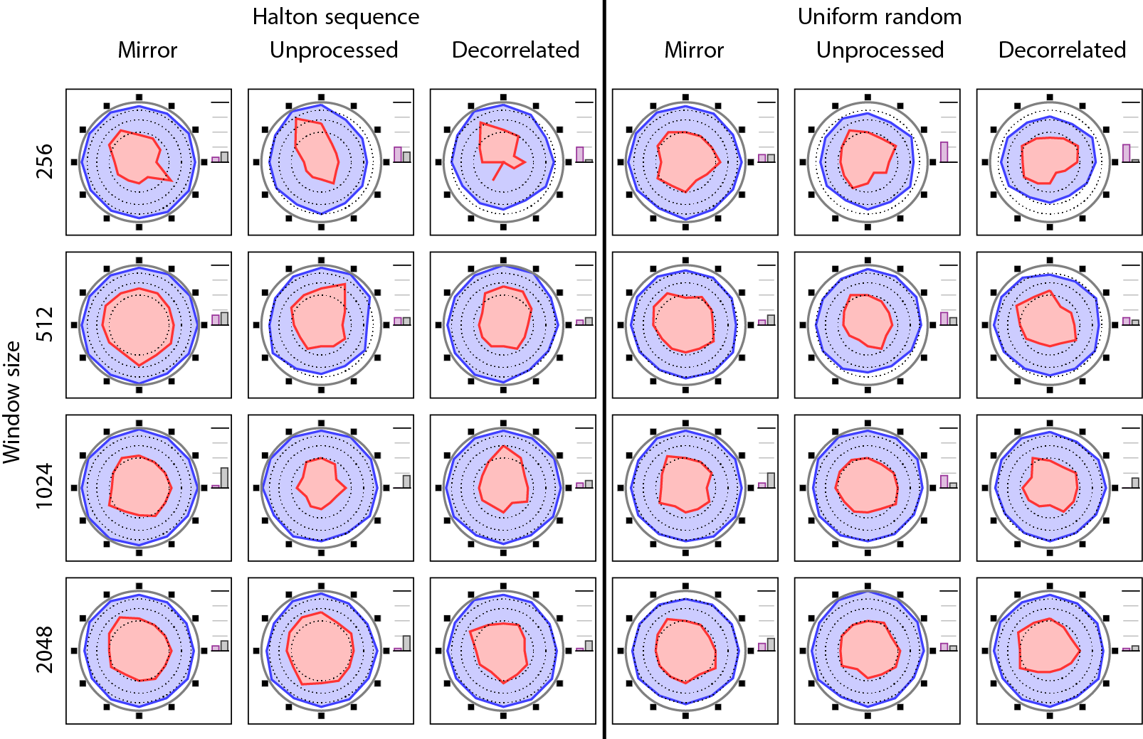
Figure: This is the result for the sample containing a cello playing in reverberant acoustics. |

Figure: This is the result for the sample containing a male speaking in dry acoustics. |
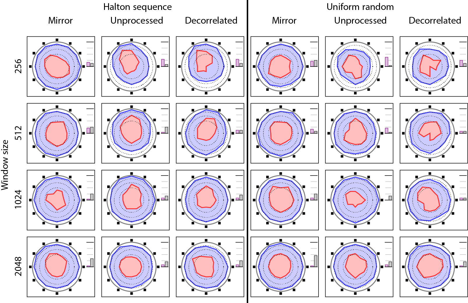
Figure: This is the result for the sample containing a recording of a sea shore. |
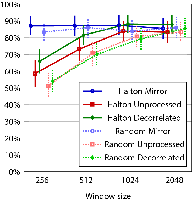
Figure: This shows the counted number of marked directions as presented in the paper. 95% confidence intervals are included. |
Results of experiment 1b
These plots show the significant effects of the variance analysis. In addition, the significant effect table is provided here.
Table: The significant effects in the variance analysis.
|
||||||||||||||||||||||||||||||||||||
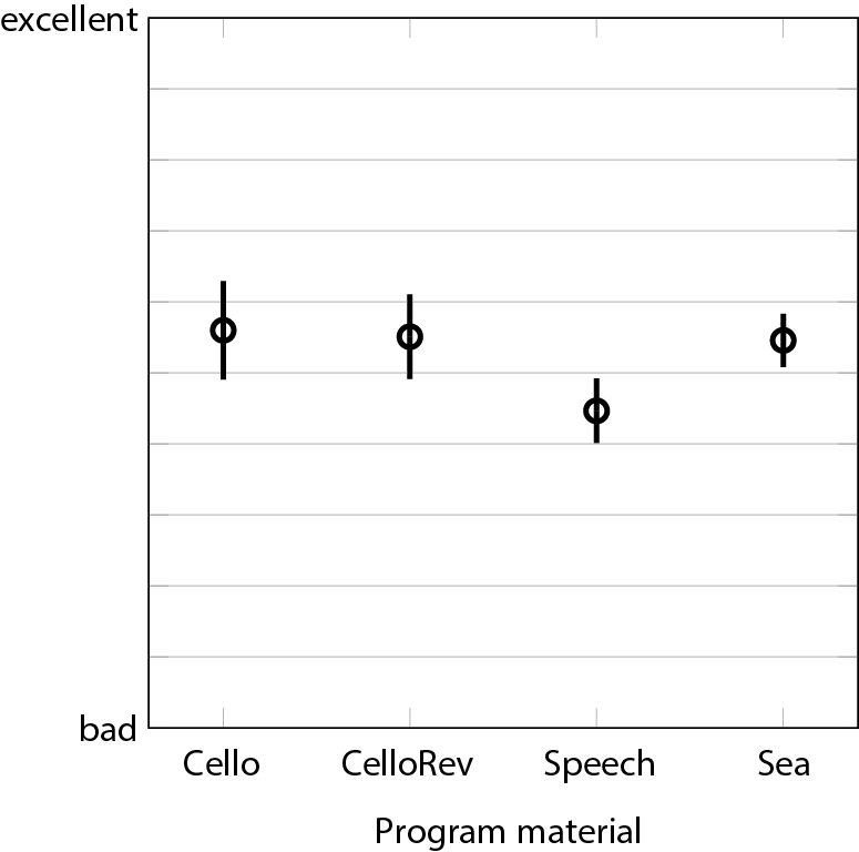
Figure: Marginal means and 95% confidence intervals for the main effect program material. |
||||||||||||||||||||||||||||||||||||
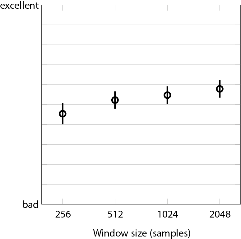
Figure: Marginal means and 95% confidence intervals for the main effect window size. |
||||||||||||||||||||||||||||||||||||
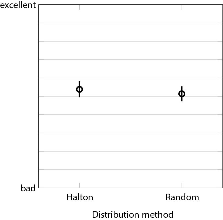
Figure: Marginal means and 95% confidence intervals for the main effect distribution method. |
||||||||||||||||||||||||||||||||||||
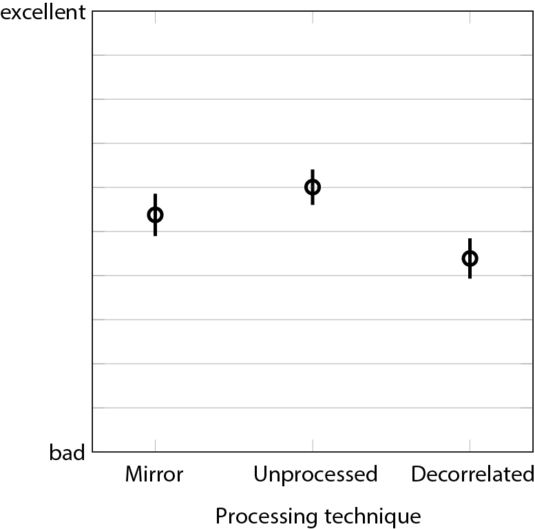
Figure: Marginal means and 95% confidence intervals for the main effect processing technique. |
||||||||||||||||||||||||||||||||||||
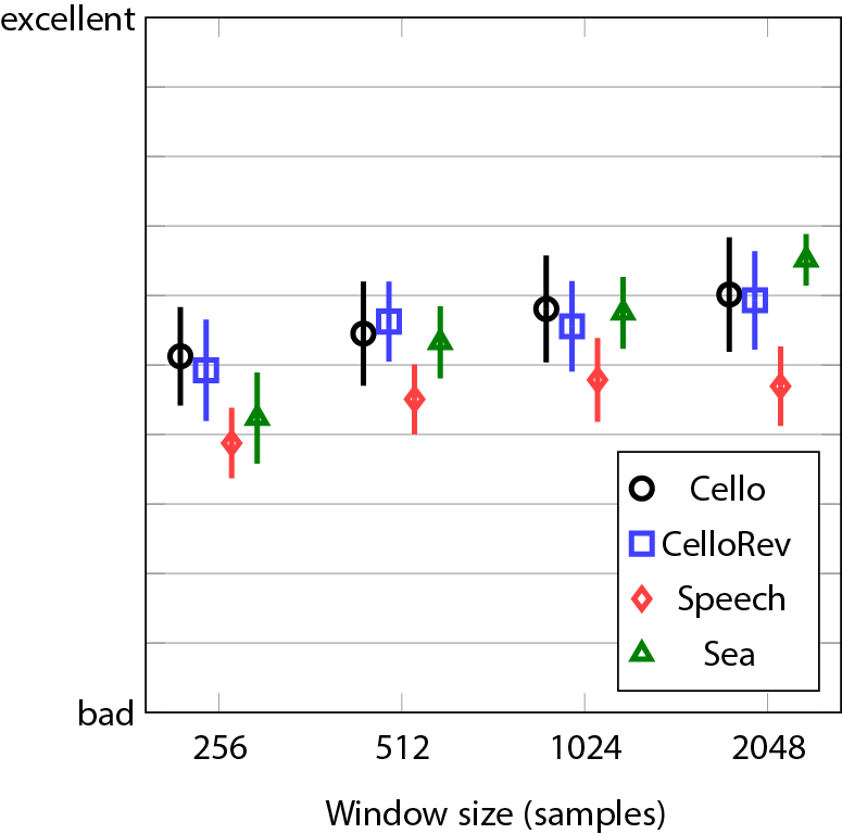
Figure: Marginal means and 95% confidence intervals for the interaction program material * window size. |
||||||||||||||||||||||||||||||||||||
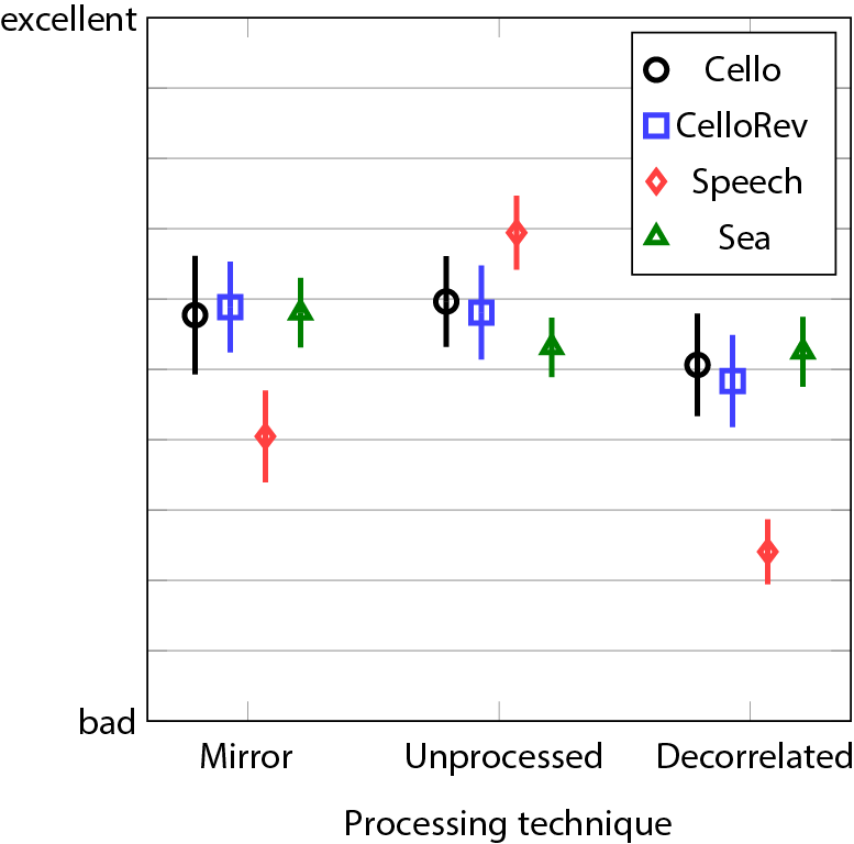
Figure: Marginal means and 95% confidence intervals for the interaction program material * processing technique. |
||||||||||||||||||||||||||||||||||||
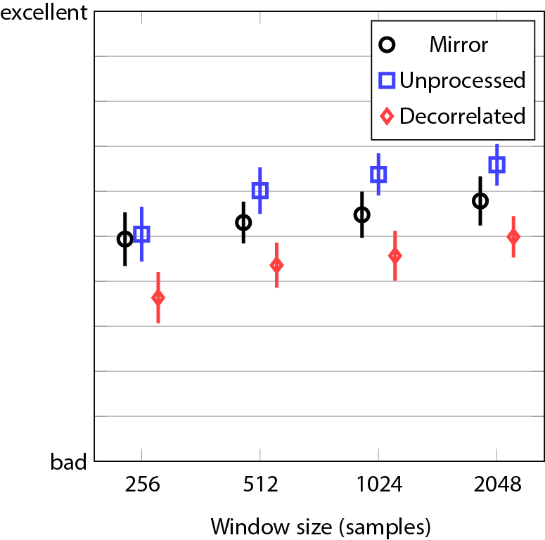
Figure: Marginal means and 95% confidence intervals for the interaction window size * processing technique. |
||||||||||||||||||||||||||||||||||||
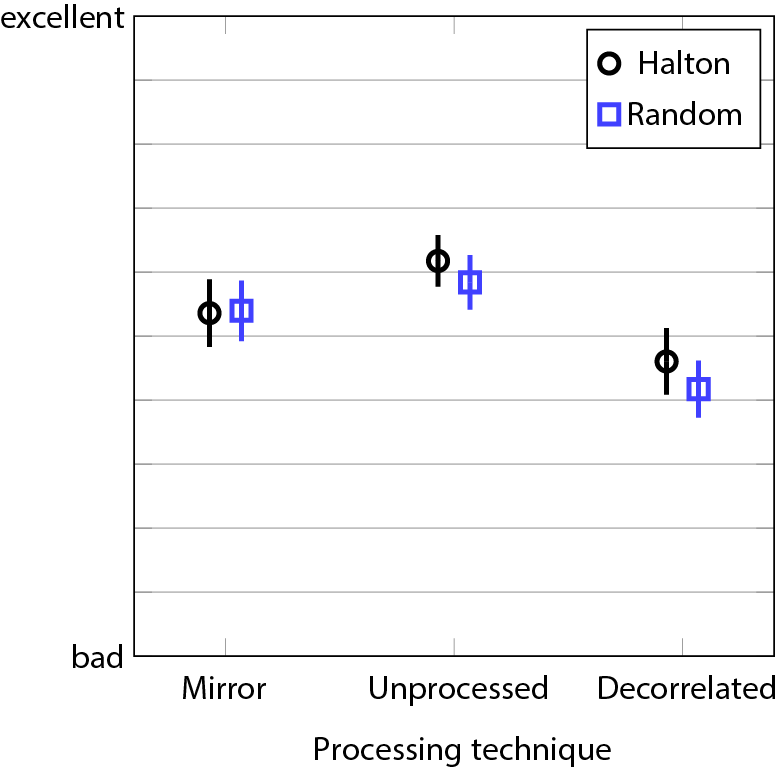
Figure: Marginal means and 95% confidence intervals for the interaction distribution method * processing technique. |
||||||||||||||||||||||||||||||||||||
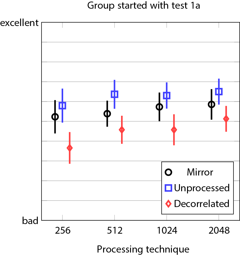
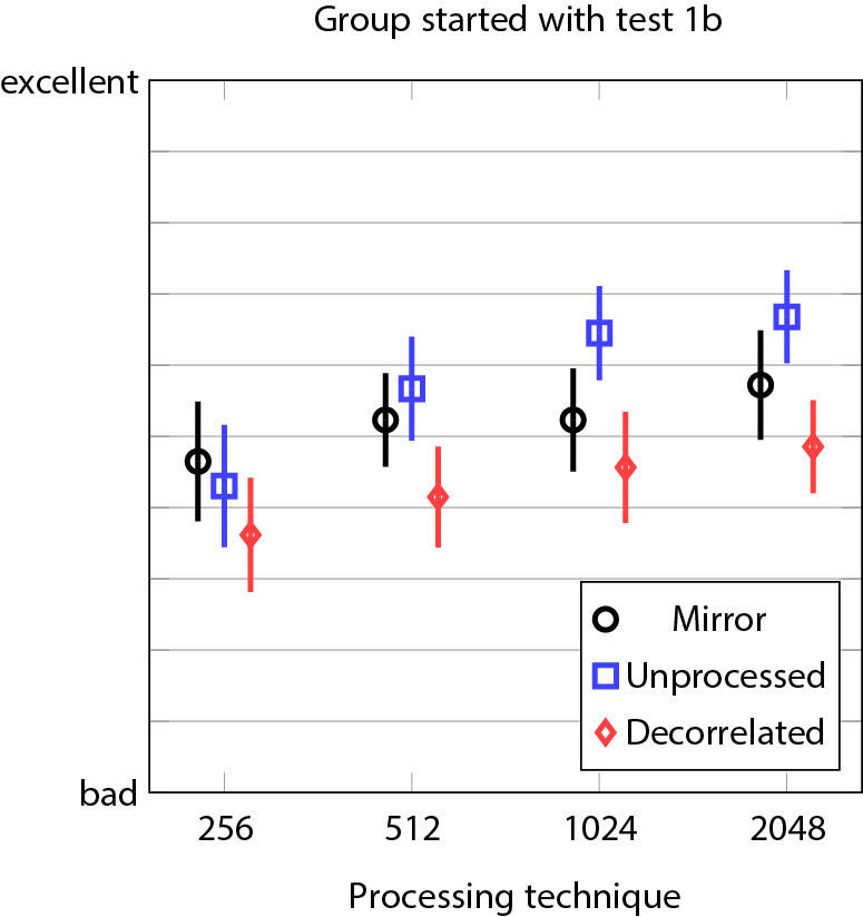
Figure: Marginal means and 95% confidence intervals for the interaction window size * processing technique * group. |
||||||||||||||||||||||||||||||||||||
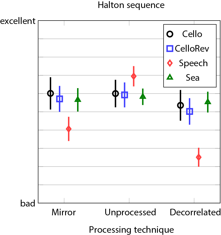
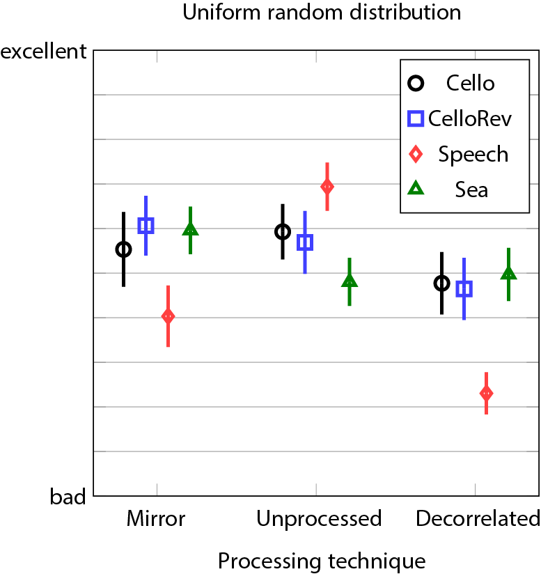
Figure: Marginal means and 95% confidence intervals for the interaction program material * distribution method * processing technique. |
||||||||||||||||||||||||||||||||||||
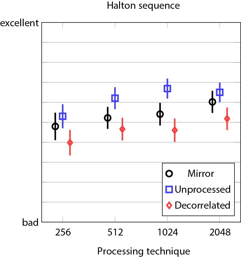
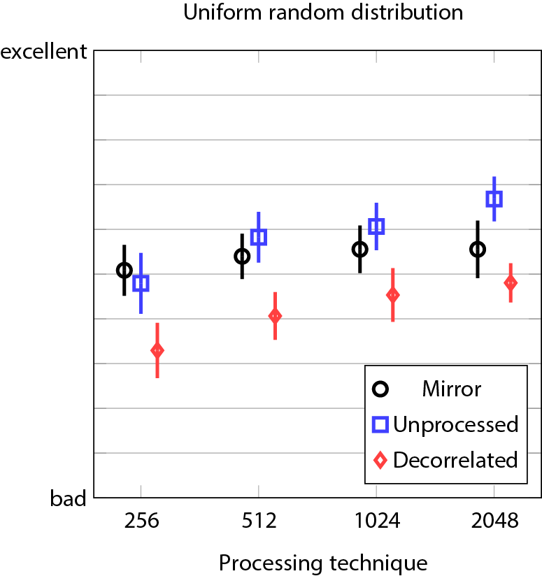
Figure: Marginal means and 95% confidence intervals for the interaction window size * distribution method * processing technique. |
Results of experiment 2
This shows the results of experiment 2 as presented in the article.
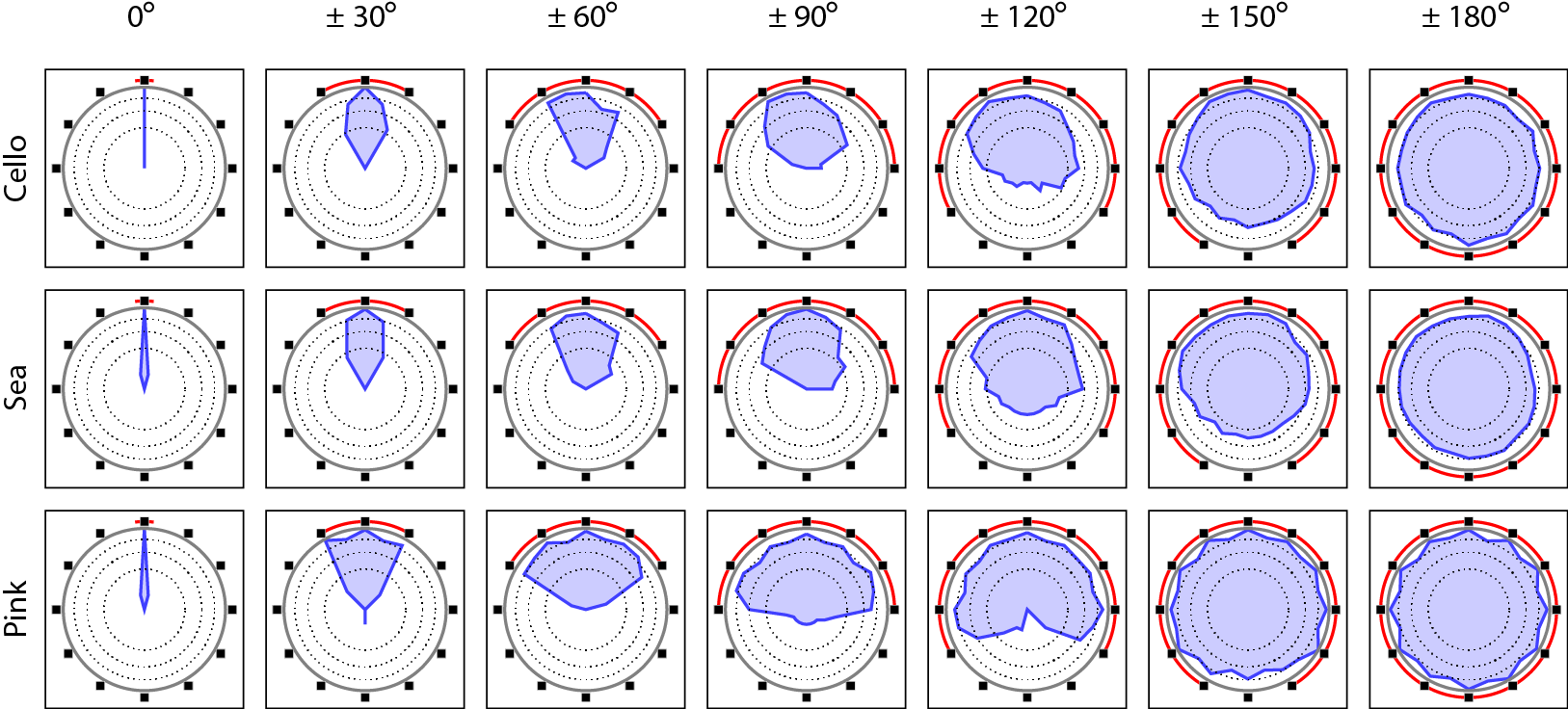
Figure: Distribution histograms for different widths. Red line signifies the area which contains the used loudspeakers while the small black boxes indicate the directions of the loudspeakers. Thick gray line is the 100% marker and dotted lines are 75%, 50%, and 25% markers. The histogram is on a square-root scale as this makes areas visually comparable. Note that it was possible to answer also between the shown loudspeakers. |
Sound examples
These sound samples provide an example of the processing. They have been processed with the spatial extent synthesis method with a mono input (provided here for comparison) and presumed 12-channel 30-degree-spaced horizontal loudspeaker setup. These loudspeaker signals have been processed with HRIRs of Kemar dummy head measured in MIT (see link). Disclaimer: These binaural renderings do not give the proper perception that is possible with a surrounding loudspeaker setup or headtracked binaural reproduction. If you want to hear the method properly with your system (and samples), please contact the first author.Effect of window size
These samples vary the window size. Otherwise, they use Halton sequence distribution and unprocessed output.- Dry cello, window size 1024 | Dry cello, window size 256 | Dry cello, mono reference
- Reverberated cello, window size 1024 | Reverberated cello, window size 256 | Reverberated cello, mono reference
- Dry male speech, window size 2048 |
Dry male speech, window size 1024 |
Dry male speech, window size 512 | Dry male speech, window size 256 |
Dry male speech, mono reference - Sea shore, window size 1024 | Sea shore, window size 256 | Sea shore, mono reference
Effect of distribution methods and techniques
The first sample set showcases all the different combinations of distribution methods and processing techniques. The window size is 1024 in all of these samples.- Reverberated cello, halton sequence, mirror |
Reverberated cello, random, mirror |
Reverberated cello, halton sequence, unprocessed | Reverberated cello, random, unprocessed |
Reverberated cello, halton sequence, decorrelated | Reverberated cello, random, decorrelated |
Reverberated cello, mono reference - Dry male speech, halton sequence, mirror |
Dry male speech, random, mirror |
Dry male speech, mono reference
http://www.acoustics.hut.fi/publications/papers/jaes-extent/
Updated on Friday February 14, 2014
This page uses HTML5, CSS, and JavaScript